38 Results
View results:
Sort by:
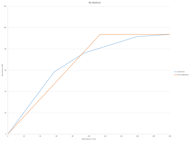
In order to be able to carry out a pushover analysis, it is necessary to transform the determined capacity curve into a simplified form. The N2 method is described in Eurocode EN 1998. This article should help to explain what a bilinearization according to the N2 method involves.
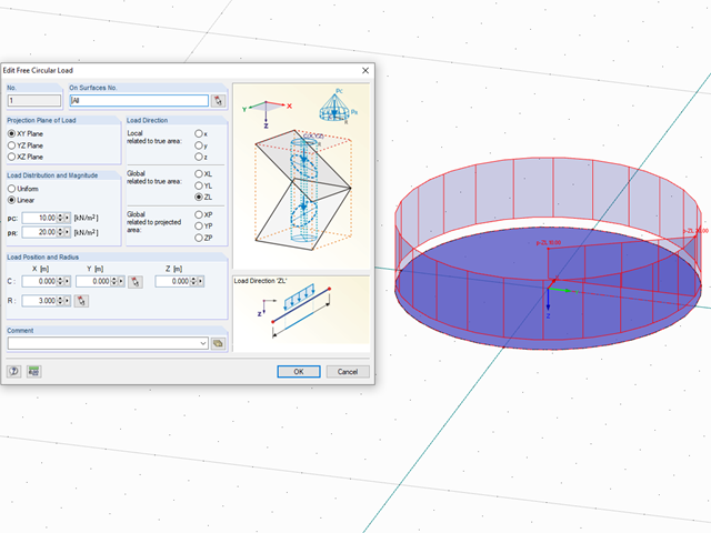
In RFEM, loads can be freely defined on surfaces. It is impossible, however, to define a variable loading on, for example, circular surfaces. However, you can still create this type of loading by using a free circular load.
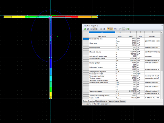
With the SHAPE‑THIN cross‑section properties software, you can create any thin‑walled cross‑section and use it in RFEM or RSTAB as a member cross‑section. SHAPE‑THIN can give all relevant cross‑section values of any cross‑section for a design and stress analysis.
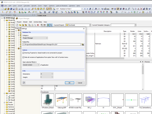
In RFEM and RSTAB, you can work with the Project Manager. It allows you to create an entire project structure and to connect it with the folders on the local hard disk.
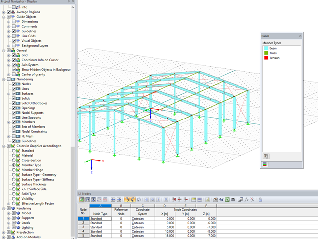
In RFEM and RSTAB, you can now also display and check the types of members used visually, by means of colors. To do this, an option has been integrated into the Display Navigator.
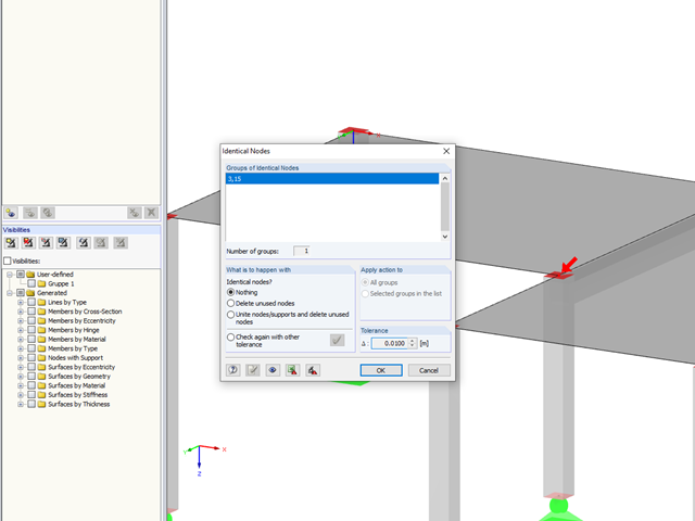
In RFEM 5 and RSTAB 8, you can save problems and warnings occurring during the model check as an extra view. This way, you can easily work through the hints and messages, one after the other, cleaning the model. The function is available for double nodes, overlapping members/lines, and surfaces.
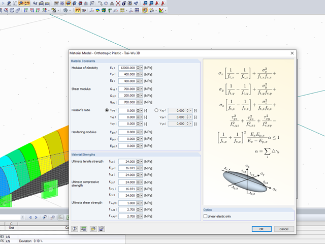
With the orthotropic elastic-plastic material model, you can calculate solids with plastic material properties in RFEM 5 and evaluate them according to the Tsai‑Wu failure criterion. The Tsai-Wu criterion is named for Stephen W. Tsai and Edward M. Wu, who published it in 1971 for plane stress states.
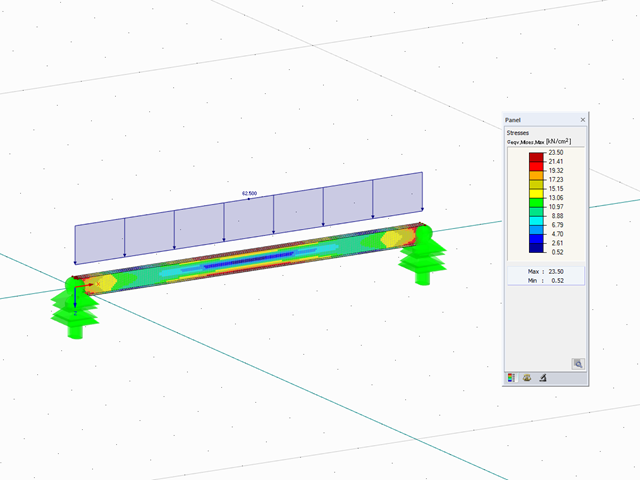
The elastic‑plastic material model in RFEM 5 allows you to calculate surfaces and solids with plastic material properties and to carry out a stress evaluation. This material model is based on the classic von Mises plasticity.
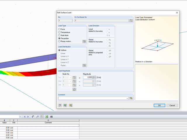
In RFEM, you have the option to consider an imperfection on surfaces. You can do this by means of the "Precamber" surface load.
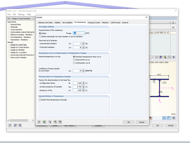
The RF-/STEEL EC3 add‑on module allows for the fire protection design of structural steel components. The simplified analysis is performed by determining the steel temperature iteratively for a particular point of time.